1.11. Parallelization of Simulation and Optimization

For the sake of simplicity, we import classes from the standard use case of rabi driving in the rotating frame with xy control, as this section focuses solely on the parallelization. (It is the same Example as in the last sections.)

1.11.1. Parallel evaluation of Monte Carlo simulations

Monte Carlo simulations can become very costly, if many noise traces are required to suppress statistical uncertainties, and the pulse needs to be sampled at very small time steps \(\delta t\) to increase the maximal noise frequency which can be resolved \(f_{max} = 1/ \delta t\).

The computational time can be reduced by performing the simulation for multiple noise samples in parallel.

import matplotlib.pyplot as plt
from qopt.examples.rabi_driving.rabi_xy_setup import *
import time

n_pulses = 10
random_pulses = np.random.rand(n_pulses, n_time_samples, len(qs_solver.h_ctrl))

monte_carlo_solver = solver_colored_noise_xy
monte_carlo_solver.set_optimization_parameters(random_pulses[0])

We start by calculating the propagators without parallelization and take the time.

monte_carlo_solver.processes = 1
start = time.time()
_ = monte_carlo_solver.propagators
end = time.time()
print('sequentiel execution')
print(end - start)

sequentiel execution
52.936718225479126

Then we continue do the same using the parallel evaluation. (We need to reset the optimization parameters, as otherwise the solver will return the stored propagators from the previous call.

monte_carlo_solver.set_optimization_parameters(0 * random_pulses[0])
monte_carlo_solver.set_optimization_parameters(random_pulses[0])

# By setting the number of processes to None, the program uses the number of
# kernels in your CPU.
monte_carlo_solver.processes = None
start = time.time()
_ = monte_carlo_solver.propagators
end = time.time()
print('parallel execution')
print(end - start)

parallel execution
18.36955976486206

1.11.2. Parallel Optimization

Gradient based optimization algorithms often require many initial values because they tend to get stuck in local minima. Fortunately this task has a trivial parallelization. We simply conduct the same optimization with different initial conditions on multiple cores.

from qopt import *

n_optimizations = 10
random_pulses = np.random.rand(
    n_optimizations, n_time_samples, len(qs_solver.h_ctrl))

start = time.time()
data = run_optimization_parallel(optimizer, initial_pulses=random_pulses,
                                 processes=None)
end = time.time()
print('parallel execution')
print(end - start)

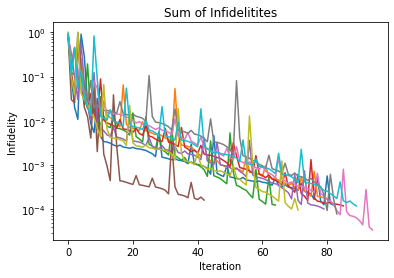
analyser = Analyser(data)
analyser.plot_absolute_costs()
plt.show()

print('Total execution time:')
print(analyser.total_cost_fkt_time() + analyser.total_grad_fkt_time())

parallel execution
100.77676844596863

Total execution time:
818.7418937683105

When performed on a 6 core CPU the parallel calculation showed a decent speedup of about a factor of 4.5.

1.11.3. Parallel Simulation

If you want to use just the Simulation tools then here you can find an example of easy parallelization using the native multiprocessing package:

from qopt.examples.rabi_driving.rabi_xy_setup import *
from multiprocessing import Pool


n_pulses = 10
random_pulses = np.random.rand(n_pulses, n_time_samples, len(qs_solver.h_ctrl))

start_parallel = time.time()
with Pool(processes=None) as pool:
    infids = pool.map(simulate_propagation, random_pulses)
end_parallel = time.time()
parallel_time = end_parallel - start_parallel

start_sequential = time.time()
infids_sequential = list(map(simulate_propagation, random_pulses))
end_sequential = time.time()
sequential_time = end_sequential - start_sequential

print('parallel execution')
print(parallel_time)
print('sequential execution')
print(sequential_time)

parallel execution
80.65793561935425
sequential execution
180.2660403251648