1.9. Filter Functions

are a great mathematical tool to calculate the influence of classical noise with a given spectral noise density on a quantum gate. Especially for small systems and high noise frequencies, the simulation with filter functions is much more efficient than a Monte Carlo simulation and more general than a Lindblad master equation.

The implementation of filter functions is imported from the package filter_functions available on github. You can find additional literature on filter functions in the following papers.

Tobias Hangleiter, P. Cerfontaine, and H. Bluhm. Filter-function formalism and software package to compute quantum processes of gate sequences for classical non-Markovian noise. Phys. Rev. Res. 3, 043047 (2021). 10.1103/PhysRevResearch.3.043047. arXiv:2103.02403.

Pascal Cerfontaine, T. Hangleiter, and H. Bluhm. Filter Functions for Quantum Processes under Correlated Noise. Phys. Rev. Lett. 127, 170403 (2021). 10.1103/PhysRevLett.127.170403. arXiv:2103.02385.

1.9.1. Example System

Lets consider the example of a singlet-triplet qubit. In this encoding of a semiconductor spin qubit, two electrons are confined in a double quantum dot subjected to a magnetic field. The computational states are the spin states of zero total spin along the quantization axis \(\vert \uparrow \downarrow>\) and \(\vert \downarrow \uparrow>\). The Hamiltonian consists is then written as

\begin{equation} H=\Delta B_z \sigma_z + J(\epsilon(t))\sigma_x \end{equation}

with the magnetic field gradient \(\Delta B_z\) across the double quantum dot and the exchange interaction \(J(\epsilon(t)) = e^{\epsilon(t)}\) depending on the difference in chemical potential \(\epsilon(t)\). This potential \(\epsilon\) is electrically controlled to drive qubit rotations while the magnetic gradient establishes the drift dynamics, and we identify the drift Hamiltonian \(H_d = \Delta B_z \sigma_z\) and the control Hamiltonian \(H_c = \sum_k u_k(t) A_k = J(\epsilon(t))\sigma_x\) with the only control amplitude \(u_1 = J(\epsilon(t))\) depending on the optimization parameter \(v=\epsilon\).

from qopt import *
import numpy as np
import matplotlib.pyplot as plt
import filter_functions as ff

delta_b_z = 2

n_time_steps = 50
delta_t = .2

def exchange_energy(epsilon):
    return np.exp(epsilon)

def deriv_exchange_energy(epsilon):
    return np.exp(epsilon)

amplitude_function = UnaryAnalyticAmpFunc(
    value_function=exchange_energy,
    derivative_function=deriv_exchange_energy
)

h_drift = [.5 * delta_b_z * DenseOperator.pauli_z()]
h_ctrl = [.5 * DenseOperator.pauli_x()]

1.9.2. Calculate Filter Functions

We will now discuss how to calculate filter functions with the qopt interface.

Any noise on the electrical control \(\epsilon(t) \rightarrow \epsilon(t) + \delta \epsilon(t)\) couples to the qubit via the noise Hamiltonian

\begin{equation} H_n= \delta \epsilon(t) \frac{\partial J(\epsilon(t))}{\partial \epsilon}\sigma_x. \end{equation}

The argument filter_function_h_n contains the noise Hamiltonian which must be of the form

\begin{equation} H_n=\sum_k s_k b_k B_k. \end{equation}

where \(s_k\) is the noise susceptibility, \(b_k\) is the noise amplitude and \(B_k\) the operator coupling to the system. In this example we just have a single term with \(s=\frac{\partial J(\epsilon(t))}{\partial \epsilon}\), \(b=\delta \epsilon\) and \(B=\sigma_x\).

The argument filter_function_h_n must be given as callable in this example, because depends on the control amplitudes and is not constant. It is given as function receiving three arguments: 1. Optimization Parameters: The parameters that are set to the solver. 2. Transferred Parameters: These are the optimization parameters after the transfer function has been applied. (See also the section about transfer functions.) 3. Control Amplitudes: These are calculated by applying the transfer function and the amplitude function. (See also the section about the amplitude function.)

In this example, we do not use a transfer function and hence the first two arguments are equal.

# The filter function noise Hamiltonian can also be set statically, if it does
# not depend on the control amplitudes.
def filter_function_h_n(opt_pars, tr_pars, ctrl_amps):
    return [[
    .5 * DenseOperator.pauli_z(),
    deriv_exchange_energy(opt_pars)[:, 0],
    'Electric Noise'
]]

In the next section, we also want to use the filter functions for optimal control and with analytic gradients, and the calculation of the derivative of the filter function needs the derivative of the noise susceptibility \(s=\frac{\partial J(\epsilon(t))}{\partial \epsilon}=\frac{\partial e^{ \epsilon(t)}}{\partial \epsilon} = e^{\epsilon(t)} = J\) by the control amplitudes, which is \(\frac{\partial s}{\partial u}=\frac{\partial J(\epsilon(t))}{\partial J(\epsilon(t))}=1\). It might feel unintuitive that we need the derivative by the control amplitudes \(\frac{\partial s}{\partial u}\) and not directly by the optimization parameter \(\frac{\partial x}{\partial v}\), but this is required by the structure of qopt, because qopt first calculates the derivatives of the cost functions by the control amplitudes and then uses automatically the transfer and the amplitude function to calculate the derivatives by the optimization parameters. This information is given to the solver in the argument filter_function_n_coeffs_deriv, which has the same signature as filter_function_h_n.

The order of the noise terms in filter_function_n_coeffs_deriv must correspond to order defined in filter_function_h_n!

def filter_function_n_coeffs_deriv(opt_pars, tr_pars, ctrl_amps):
    derivatives = np.ones_like(opt_pars)
    derivatives = np.expand_dims(derivatives.T, axis=0)  # Additional axis for
    # the number of noise operators
    return derivatives

solver = SchroedingerSolver(
    h_drift=h_drift,
    h_ctrl=h_ctrl,
    tau=delta_t * np.ones(n_time_steps),
    amplitude_function=amplitude_function,
    filter_function_h_n=filter_function_h_n,
    filter_function_n_coeffs_deriv=filter_function_n_coeffs_deriv
)
np.random.seed(0)
ctrl_amplitudes = np.random.rand(n_time_steps, 1) - .5
solver.set_optimization_parameters(ctrl_amplitudes)

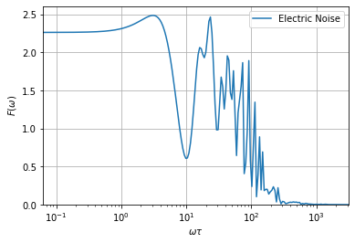
We can create an instance of the PulseSequence class, and use all the functionalities of the filter_functions package:

solver.create_pulse_sequence()
pulse_sequence = solver.pulse_sequence
omega = ff.util.get_sample_frequencies(
    pulse_sequence, n_samples=200, spacing='log')
_ = ff.plotting.plot_filter_function(pulse_sequence, omega)

But the calculation of the infidelity is also completely capsulated by the cost function OperatorFilterFunctionInfidelity, which also holds the information about the power spectral density of our noise souce:

\begin{equation} S(f) = \int <b(0) b(t)> e^{2 \pi f t} dt = \int <\delta \epsilon(0) \delta \epsilon(t)> e^{2 \pi f t} dt \end{equation}

def psd(f):
    return 1e-3/f

ff_infid = OperatorFilterFunctionInfidelity(
    solver=solver,
    noise_power_spec_density=psd,
    omega=omega,
    label=['FF Infidelity', ]
)
ff_infid.costs()

array([0.01302111])

1.9.3. Optimal Control with Filter Functions

With the implementation of Analytic Filter-Function Derivatives for Quantum Optimal Control, filter functions are available as efficient tool in quantum optimal control. The derivatives allow us to optimize pulses with cost functions defined by filter functions. This enables the numeric calculations of pulses that are especially robust towards noise of specific frequencies.

Isabel N. M. Le, J. D. Teske, T. Hangleiter, P. Cerfontaine, and Hendrik Bluhm. Analytic Filter Function Derivatives for Quantum Optimal Control. Phys. Rev. Applied 17, 024006 (2022). 10.1103/PhysRevApplied.17.024006. arXiv:2103.09126.

Optimal control with filter functions can also be used in noise spectroscopy since it is possible to optimize pulses to be susceptibile to a specific noise frequency.

We optimize a pulse for the example above:

# We need to add another cost function to set a target gate for the coherent
# evolution in the absence of noise.
coherent_costs = OperationInfidelity(
    solver=solver,
    target=DenseOperator.pauli_x()
)

simulator = Simulator(
    solvers=[solver, ],
    cost_funcs=[ff_infid, coherent_costs]
)

It is always a good advice to check the implementation of derivatives by comparing the analytic to numeric gradients. The Simulator has a convenience function to calculate the absolute and relative deviation of both:

print(simulator.compare_numeric_to_analytic_gradient(ctrl_amplitudes))

(5.460480386219424e-08, 1.82142191149408e-07)

From the comparison of analytic and numeric gradients, we know that our implementation is correct. Next we optimize the pulse.

optimizer = ScalarMinimizingOptimizer(
    system_simulator=simulator
)
result = optimizer.run_optimization(ctrl_amplitudes)

Lets plot the results of the optimization:

data = DataContainer()
data.append_optim_result(result)
analyser = Analyser(data)
analyser.plot_costs()

<AxesSubplot:xlabel='Iteration', ylabel='Costs'>

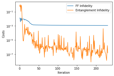
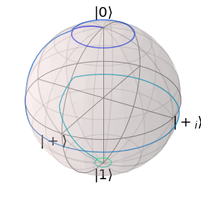
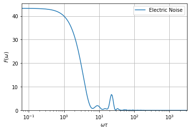
The Infidelity contribution of the 1/f-noise has dropped substantially. We plot again the filter function and the pulse.

pulse_sequence2 = solver.create_pulse_sequence(result.final_parameters)
ff.plotting.plot_filter_function(pulse_sequence2, omega)

solver.plot_bloch_sphere()