1.10. Energy Spectra

A convenience feature for the analysis of quantum systems is a module for plotting the energy spectrum of a quantum system described by a Hamilton \(H\) operator. The energy spectrum itself is the set of eigenvalues \(\{e_i\}_i\) as function of a control parameter \(\epsilon\).

As an example application, we study low energy states in two quantum dots, starting with the Hamiltonian

\begin{equation} H(\epsilon) = \epsilon \tau_z \end{equation}

where the control parameter is the detuning \(\epsilon\) and \(\tau_z\) is the pauli matrix on the charge space spanned by the basis vectors \(\vert L \rangle\) and \(\vert R \rangle\).

import numpy as np
import matplotlib.pyplot as plt
from qopt.matrix import DenseOperator
from qopt.energy_spectrum import plot_energy_spectrum

pauli_z = DenseOperator.pauli_z()
pauli_x = DenseOperator.pauli_x()
detuning_range = np.linspace(-2, 2, 100)
hamiltonians = [eps * pauli_z for eps in detuning_range]

plot_energy_spectrum(hamiltonian=hamiltonians, x_val=detuning_range,
                     x_label='Detuning in eV')
plt.show()

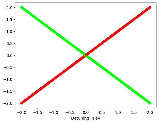
The points mark the eigenvalues of the Hamiltonian and the colors encode the contribution of the basis states to the eigenvectors. We observe a crossing without mixing of the eigenvectors. Lets now add a tunnel coupling \(t_c\) to the Hamiltonian:

\begin{equation} H(\epsilon) = \epsilon \tau_z + t_c \tau_x \end{equation}

t_c = .5
hamiltonians_tc = [eps * pauli_z + t_c * pauli_x for eps in detuning_range]

plot_energy_spectrum(hamiltonian=hamiltonians_tc, x_val=detuning_range,
                     x_label='Detuning in eV')
plt.show()

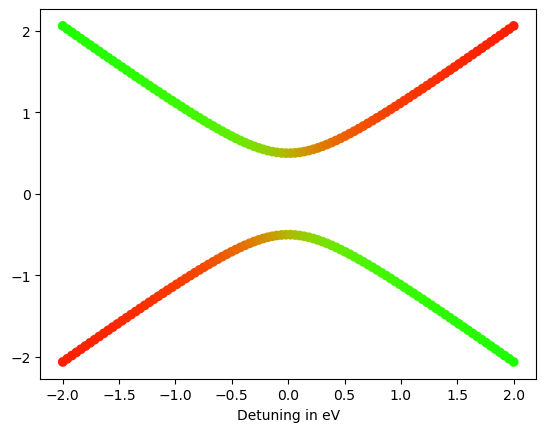
Here we observe an avoided crossing around which the eigenvectors are mixing, shown by the brownish color. Now lets add the spin subspace and introduce a magnetic field along the quantization axis, resulting in a Zeeman energy \(E_z\).

\begin{equation} H(\epsilon) = \epsilon \tau_z + t_c \tau_x + E_z \sigma_z \end{equation}

Here \(\sigma_z\) denotes the pauli operator on the spin space spanned by the states \(\vert \uparrow \rangle\) and \(\vert \downarrow \rangle\). Thus the total Hilbertspace is the productspace of the charge and spin space.

tau_z = pauli_z.kron(pauli_z.identity_like())
tau_x = pauli_x.kron(pauli_x.identity_like())
sigma_z = pauli_x.identity_like().kron(pauli_z)

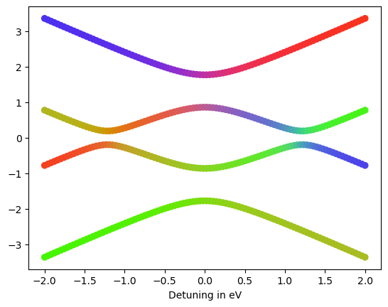
E_z = 1.2
hamiltonians_tc_E_z = [
    eps * tau_z + t_c * tau_x + E_z * sigma_z
    for eps in detuning_range
]

plot_energy_spectrum(hamiltonians_tc_E_z, x_val=detuning_range,
                     x_label='Detuning in eV')
plt.show()

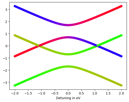
And we can create two additional avoided crossings, if we include a magnetic field gradient \(B_x\):

\begin{equation} H(\epsilon) = \epsilon \tau_z + t_c \tau_x + E_z \sigma_z + B_x \sigma_x \tau_z \end{equation}

sigma_x = pauli_x.identity_like().kron(pauli_x)

B_x = .5
hamiltonians_tc_E_z_B_x = [
    eps * tau_z + t_c * tau_x + E_z * sigma_z + B_x * sigma_x * tau_z
    for eps in detuning_range
]

plot_energy_spectrum(hamiltonians_tc_E_z_B_x, x_val=detuning_range,
                     x_label='Detuning in eV')
plt.show()