1.8. Simulation of open quantum systems
Schroedinger’s equation describes closed quantum where all dynamics are unitary and hence reversible. To simulate the loss of information caused by relaxation effects, we can describe the system as open quantum system with a master equation in Lindblad form:
We come back to the example of a single qubit under rabi driving, but this time we take relaxations into the ground state into account, leading to a relaxation quantified by the so called \(T_1\)-time or depolarization time.
The Hamiltonian is given by:
And the Lindblad operator, which describes the dissipative effects:
where \(\gamma = 1 / T_1\) is the depolarization rate and the descending operator
[1]:
import numpy as np
import matplotlib.pyplot as plt
from qopt import *

sigma_x = DenseOperator.pauli_x()
sigma_y = DenseOperator.pauli_y()
sigma_z = DenseOperator.pauli_z()
sigma_minus = DenseOperator.pauli_m()
zero_matrix = DenseOperator(np.zeros((2, 2)))

h_ctrl = [.5 * sigma_x, .5 * sigma_y]
h_drift = [zero_matrix]
The master equation can be linearized with the Kronecker product, for which holds:
The linearized form of the master equation is then:
with
and the dissipation operator
The master equation can be implemented in two different ways. Either we define the Lindblad operators and their corresponding prefactors, or we construct the dissipation operator.
Lets discuss the former option and assume that the relaxation rate is proportional to the driving amplitude:
The \(u\) are control amplitudes \(u_x = A \text{cos}( \delta )\) and \(u_y = A \text{sin}(\delta)\). Making them appear in the Lindblad equations creates the possibility to minimize the dissipation by changing the control amplitudes.
[2]:
lindblad_operators = [sigma_minus, ]
gamma_0 = .001

# The required signature of the prefactor function can be found in
# the API documentation of the LindbladSolver.
def prefactor_function(control_amplitudes, *_):
    return gamma_0 * np.expand_dims(
        np.sum(np.abs(control_amplitudes), axis=1), axis=1)


def prefactor_function_derivative(control_amplitudes, *_):
    return np.expand_dims(gamma_0 * np.sign(control_amplitudes), axis=2)
The prefactor function now returns the depolarization rate \(\gamma\), which is the squared amplitude of the lindblad operator. The simulation package assumes that the Lindblad operators can be given as constant operator \(L_k\), which is multiplied with a prefactor \(c_k\) to calculate the dissipation operator as:
The derivatives of the prefactor function must be implemented as well if the derivative of the cost function shall be calculated.
Now we can instantiate the solver and cost function.
[3]:
total_time = 1
n_time_steps = 5
time_steps = (total_time / n_time_steps) * np.ones((n_time_steps, ))

solver = LindbladSolver(
    h_drift=h_drift,
    h_ctrl=h_ctrl,
    tau=time_steps,
    lindblad_operators=lindblad_operators,
    prefactor_function=prefactor_function,
    prefactor_derivative_function=prefactor_function_derivative
)

x_half = sigma_x.exp(np.pi * .25j)

entanglement_infid = OperationInfidelity(
    solver=solver,
    target=x_half,
    super_operator_formalism=True
)
Please note that we have to set the option super_operator_formalism in the cost function to True. Next we optimize the control amplitudes.
[4]:
simulator = Simulator(
solvers=[solver],
cost_funcs=[entanglement_infid]
)
termination_conditions = {
"min_gradient_norm": 1e-15,
"min_cost_gain": 1e-15,
"max_wall_time": 120.0,
"max_cost_func_calls": 1e6,
"max_iterations": 10000,
"min_amplitude_change": 1e-8
}
upper_bounds = 5 * 2 * np.pi * np.ones((len(h_ctrl) * n_time_steps, ))
lower_bounds = -1 * upper_bounds
optimizer = LeastSquaresOptimizer(
system_simulator=simulator,
termination_cond=termination_conditions,
save_intermediary_steps=True,
bounds=[lower_bounds, upper_bounds]
)
np.random.seed(0)
initial_pulse = np.pi * 2 * (np.random.rand(n_time_steps, len(h_ctrl)) - 1)
result = optimizer.run_optimization(initial_control_amplitudes=initial_pulse)
solver.set_optimization_parameters(result.final_parameters)
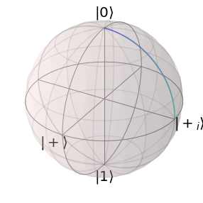
solver.plot_bloch_sphere()
plt.show()
To verify that the implemented derivatives of the prefactor function is correct, we can compare our derivatives with finite differences. The convenience function compare_numeric_to_analytic_gradient calculates the absolute and relative difference to the finite difference gradient.
[5]:
simulator.compare_numeric_to_analytic_gradient(initial_pulse)
[5]:
(1.633248503059409e-08, 9.851677024373317e-08)