1.7. Monte Carlo Simulations

The noise present in quantum mechanical systems can be described semi-classically by including random variables into Schroedinger’s equation turning it into a stochastic differential equation.

This equation can then be solved numerically with a Monte Carlo Method by sampling the noise distribution and repeating the simulation for each noise sample. In the simulation we distinguish between the general case of fast noise with a real valued spectral noise density \(S(f)\) and approximately quasi static noise. The latter describes the case where the spectral noise density is only larger than zero at frequencies which are slower than the quantum gate, i.e. \(S(f) = 0 \; \forall f > 1/T\) where \(T\) is the total gate time.

In the previous example of rabi driving, realistic experiments show some instability in the resonance frequency. Let us therefore assume that the resonance frequency of our system is time dependent as has a mean value of \(\omega_0\).

\begin{equation} \omega(t) = \omega_0 + \delta_\omega (t) \end{equation}

Then we consider the following Hamilton operator in the rotating wave approximation:

\begin{equation} H = \delta_\omega (t) \sigma_z / 2 + A_x (t) \sigma_x / 2 + A_y(t) \sigma_y / 2 \end{equation}

1.7.1. Quasi Static Noise

The noise realizations required for the Monte Carlo simulations are created in the NoiseTraceGenerator classes. Let us consider the case of quasi-static noise first:

from qopt import *
import numpy as np
import matplotlib.pyplot as plt

ntg_quasi_static = NTGQuasiStatic(
    n_samples_per_trace=10,
    standard_deviation=[.5],
    n_traces=5,
    always_redraw_samples=False,
    sampling_mode='uncorrelated_deterministic'
)

The NTGQuasiStatic receives a standard deviation for each random variable. For quasi static noise it is usually sufficient to sample only a few traces, while many more are required to suppress the statistical uncertainties for general noise spectral densities.

In the sampling mode sampling_mode='uncorrelated_deterministic' the noise is sampled deterministically from a Gaussian distribution and each variable is sampled separately. Hence, the number of noise traces which are returned are n_traces times the number of random variables.

The other implemented sampling mode is monte_carlo, where the noise traces are created with help of random number generators and all random variables are sampled simultaneously.

Next, we optimize the pulse subjected to quasi-static noise. We begin with the same setup as in the noiseless case:

sigma_x = DenseOperator.pauli_x()
sigma_y = DenseOperator.pauli_y()
sigma_z = DenseOperator.pauli_z()

delta_omega = 0

h_ctrl = [.5 * sigma_x, .5 * sigma_y]
h_drift = [delta_omega * .5 * sigma_z]

n_time_steps = 10
total_time = 1

time_steps = (total_time / n_time_steps) * np.ones((n_time_steps, ))

But we use a Monte Carlo solver.

solver_qs_noise = SchroedingerSMonteCarlo(
    h_drift=h_drift * n_time_steps,
    h_ctrl=h_ctrl,
    h_noise=[sigma_z],
    initial_state=DenseOperator(np.eye(2)),
    noise_trace_generator=ntg_quasi_static,
    tau=time_steps
)

For the cost function, we have multiple options. We can use a cost function which averages the entanglement infidelity \(F_e\) over the noise realizations to calculate the infidelity caused by noise \(\bar{F}_e\):

\begin{equation} \bar{F}_e = \frac{1}{n_\text{traces}}\sum_{\delta_\omega} F_e(\delta_\omega), \end{equation}

where \(F_e(\delta_\omega)\) is the infidelity evaluated for the evolution with the noise value \(\delta_\omega\).

This includes the stochastic (caused by noise) and the systematic (also appearing in the absence of noise) deviations. However, there are certain advantages, if the stochastic and the systematic deviations are split. It gives us a feeling for the cause of infidelities in our system, and the optimization algorithms acquires the information, that it optimizes two cost functions at once, if a vector valued optimization algorithm is chosen.

x_half = sigma_x.exp(np.pi * .25j)

entanglement_infidelity = OperationInfidelity(
    solver=solver_qs_noise,
    target=x_half
)

qs_noise_cost = OperationNoiseInfidelity(
    solver=solver_qs_noise,
    target=x_half,
    neglect_systematic_errors=True
)

We need to add the new solver and cost function to the simulator. We then also increase the maximal wall time since the Monte Carlo simulation is numerically more complex.

from qopt.simulator import Simulator
from qopt.optimize import LeastSquaresOptimizer
simulator = Simulator(
    solvers=[solver_qs_noise],
    cost_funcs=[entanglement_infidelity, qs_noise_cost]
)
# There are two cost functions connected to a single solver. We could also
# use a second solver only calculating the noiseless evolution, but this
# functionality is also included in the SchroedingerSMonteCarlo class.

termination_conditions = {
    "min_gradient_norm": 1e-15,
    "min_cost_gain": 1e-15,
    "max_wall_time": 120.0,
    "max_cost_func_calls": 1e6,
    "max_iterations": 1000,
    "min_amplitude_change": 1e-8
}

upper_bounds = 5 * 2 * np.pi * np.ones((len(h_ctrl) * n_time_steps, ))
lower_bounds = -1 * upper_bounds

optimizer = LeastSquaresOptimizer(
    system_simulator=simulator,
    termination_cond=termination_conditions,
    save_intermediary_steps=True,
    bounds=[lower_bounds, upper_bounds]
)

np.random.seed(0)
initial_pulse = np.pi * np.random.rand(n_time_steps, len(h_ctrl))

result = optimizer.run_optimization(initial_control_amplitudes=initial_pulse)
solver_qs_noise.set_optimization_parameters(result.final_parameters)
solver_qs_noise.plot_bloch_sphere()
plt.show()

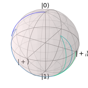
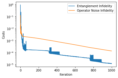
The optimized pulses are not susceptible to quasi static noise. For visualization, we can plot the cost functions during the optimization.

data_container = DataContainer(
    storage_path=r'..\..\..\temp',
    file_name="File Name"
)

data_container.append_optim_result(optim_result=result)
analyser = Analyser(data=data_container)
analyser.plot_costs()
plt.show()

1.7.2. Fast Noise

To discuss the general case of arbitrary noise spectra, lets consider the example of Johnson noise, which we directly apply to the control parameters.

The frequency range of the noise sampling is limited by the time discretization. The lower limit is \(f_{min} = 1/T\) where \(T\) is the total time of the pulse, and the upper limit is given by \(f_{max} = 1 / \delta t\), where \(\delta t\) is the spacing of the time steps. To extend \(f_{max}\) to higher values, we can use a simple transfer function, which does nothing but oversampling the pulse.

oversampling = 100
def noise_spectral_density(f):
    return 1 / f

ntg_1_over_f = NTGColoredNoise(
    noise_spectral_density=noise_spectral_density,
    dt=time_steps[0] / oversampling,
    n_samples_per_trace=n_time_steps * oversampling,
    n_traces=100,
    n_noise_operators=2
)

oversampling_tf = OversamplingTF(
    oversampling=oversampling,
    num_ctrls=2
)
oversampling_tf.set_times(time_steps)

As we apply the noise directly to the optimization parameters we can use the class SchroedingerSMControlNoise, which also automatically takes the amplitude function into account, if any is given.

solver_1_over_f = SchroedingerSMCControlNoise(
    h_drift=h_drift,
    h_ctrl=h_ctrl,
    noise_trace_generator=ntg_1_over_f,
    tau=total_time / n_time_steps * np.ones(
        (n_time_steps, )
    ),
    transfer_function=oversampling_tf
)

cost_1_over_f = OperationNoiseInfidelity(
    solver=solver_1_over_f,
    target=None,
    neglect_systematic_errors=True
)

solver_1_over_f.set_optimization_parameters(result.final_parameters)
cost_1_over_f.costs()

0.09589564915442621