2.4. \(T_2\) Dephasing with Markovian Noise
The opposite of (fully correlated) quasi-static noise is white noise. In this case, the noise traces are uncorrelated in time and hence, Markovian. Instead of performing Monte Carlo simulations to find the average evolution, we can effectively describe the effect of Markovian noise using the Lindblad master equation.
As an example, we investigate again resonant driving with the Hamiltonian
this time with fast noise terms that affect the rabi and the resonance frequency, and omit the Y-drive once again.
In this case, the Lindblad equation
has Lindblad operators \(L_1 = \frac{1}{2} \sigma_x\) and \(L_2 = \frac{1}{2} \sigma_z\) with prefactors \(\gamma_1 = \frac{1}{2} S_{x}\) and \(\gamma_2 = \frac{1}{2} S_{\omega}\). Here, \(S_{i}\) is the one-sided noise spectral density (NSD) which is defined as one half of Fourier transformed auto-correlation function \(\langle \delta_i(\Delta t)\delta_i(0) \rangle\) where \(\delta_i(t)\) is the noise on the parameter \(i\) (\(\in \{x, \omega\}\) in our case). The factor \(\frac{1}{2}\) rescales the NSD to its two-sided pendant.
[1]:
import numpy as np
import matplotlib.pyplot as plt

from qopt.matrix import DenseOperator
from qopt.solver_algorithms import LindbladSolver

pauli_0 = DenseOperator.pauli_0()
pauli_x = DenseOperator.pauli_x()
pauli_y = DenseOperator.pauli_y()
pauli_z = DenseOperator.pauli_z()

nsd_drive = .2
nsd_resonance = 1.5
n_time_steps = 200
total_time = 10
rabi_frequency = 2 * np.pi

def create_lindblad_solver(noise_spectral_density_drive,
                           noise_spectral_density_resonance):

    def prefactor_function(transferred_parameters, _):
        """
        Sets the prefactors gamma_i in the Lindblad
        equation.
        """
        prefactors = np.ones((len(transferred_parameters), 2))
        prefactors[:, 0] = .5 * noise_spectral_density_drive
        prefactors[:, 1] = .5 * noise_spectral_density_resonance
        return prefactors

    solver = LindbladSolver(
        h_drift=[0 * pauli_z, ],
        h_ctrl=[.5 * pauli_x, ],
        lindblad_operators=[.5 * pauli_x, .5 * pauli_z],
        prefactor_function=prefactor_function,
        tau=(total_time / n_time_steps) * np.ones(n_time_steps)
    )

    control_amplitude = rabi_frequency * np.ones((n_time_steps, 1))
    solver.set_optimization_parameters(control_amplitude)

    return solver
Again, we need to vectorize the density matrix for compatibility with the forward propagators that are calculated by the Lindblad solver. Hence, we define:
[2]:
def vectorize(rho):
    """Vectorizes a density matrix. """
    d_square = int(rho.shape[0] ** 2)
    return DenseOperator(np.reshape(rho.data.T, (d_square, 1)))

def devectorize(rho_vec):
    """Calculates the regular matrix expression from a vectorized matrix. """
    d = int(np.round(np.sqrt(rho_vec.shape[0])))
    return DenseOperator(np.reshape(rho_vec.data, (d, d)).T)
Next, we calculate the Bloch vector components \(v_i\), which correspond to the Pauli matrix expectation values \(\langle \sigma_i \rangle (t) = \text{Tr} \left[\sigma_i \rho(t) \right]\):
[3]:
def evaluate_bloch_components(
    forward_propagators,
    v_x, v_y, v_z
):
    init_density = 0.5 * (
            pauli_0 + v_x * pauli_x + v_y * pauli_y + v_z * pauli_z)
    init_super_vector = vectorize(init_density)

    bloch_vector_evolution = np.zeros((len(forward_propagators), 3))

    for i, propagator in enumerate(forward_propagators):
        current_density = devectorize(propagator * init_super_vector)
        bloch_vector_evolution[i,0] = np.real((pauli_x * current_density).tr())
        bloch_vector_evolution[i,1] = np.real((pauli_y * current_density).tr())
        bloch_vector_evolution[i,2] = np.real((pauli_z * current_density).tr())

    return bloch_vector_evolution
2.4.1. Noise on Rabi Frequency
The Bloch vector \(\vec{v}(t)\) of a density matrix \(\rho = \frac{1}{2} \left(\mathbb{1} + \vec{v} \cdot \vec{\sigma} \right)\) will evolve according to
At this point, we can assign the characteristic decay time \(T_2 = \frac{4}{S_x}\). For an initial up state \(\left( v_x = v_y = 0, v_z = 1 \right)\) we get
[4]:
solver_rabi_noise = create_lindblad_solver(
    noise_spectral_density_resonance=0,
    noise_spectral_density_drive=nsd_drive
)

bloch_rabi_noise = evaluate_bloch_components(
    solver_rabi_noise.forward_propagators,
    0, 0, 1
)

times = np.arange(n_time_steps + 1) * total_time / n_time_steps

T2_expected = 2 / (nsd_drive * 0.5)
decay_envelope = np.exp(-times / T2_expected)


plt.plot(times, bloch_rabi_noise[:,0], label="$\langle \sigma_x \\rangle$")
plt.plot(times, bloch_rabi_noise[:,1], label="$\langle \sigma_y \\rangle$")
plt.plot(times, bloch_rabi_noise[:,2], label="$\langle \sigma_z \\rangle$")
plt.plot(times, decay_envelope, linestyle="--", label="$\exp(-t/T_2)$")
plt.ylabel("$\langle \sigma_i \\rangle$", fontsize=12)
plt.xlabel("time / ms", fontsize=12)
plt.legend()
plt.show()
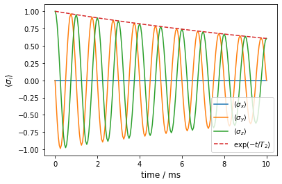
We recognize the expected behaviour and also see that it is qualitatively different from the case of quasi-static noise.
2.4.2. Noise on Resonace Frequency
For this particular case, the Bloch vector components will evolve according to
neglecting quadratic orders in \(\frac{\gamma}{4 u_s}\).
[5]:
solver_resonance_noise = create_lindblad_solver(
    noise_spectral_density_resonance=nsd_resonance,
    noise_spectral_density_drive=0
)

bloch_resonance_noise = evaluate_bloch_components(
    solver_resonance_noise.forward_propagators,
    0, 0, 1
)

times = np.arange(n_time_steps + 1) * total_time / n_time_steps

T2_expected_yz = 4 / (nsd_resonance * 0.5)

decay_envelope_yz = np.exp(-times / T2_expected_yz)


plt.plot(times, bloch_resonance_noise[:,0],
         label="$\langle \sigma_x \\rangle$")
plt.plot(times, bloch_resonance_noise[:,1],
         label="$\langle \sigma_y \\rangle$")
plt.plot(times, bloch_resonance_noise[:,2],
         label="$\langle \sigma_z \\rangle$")
plt.plot(times, decay_envelope_yz, linestyle="--",
         label="$\exp(-t/T_{2,yz})$")
plt.ylabel("$\langle \sigma_i \\rangle$", fontsize=12)
plt.xlabel("time / ms", fontsize=12)
plt.legend()
plt.show()
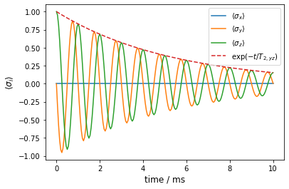
Again, we have an exponential decay which is qualitatively different from the quasi-static pendant. Generally, exponential decays of probability amplitudes are an inherent property of the Lindblad master equation due to the assumption of Markovian processes that govern the dissipative part of the evoulution (c.f., these lecture notes).