2.7. Phase Noise with Filter Functions

In this section we discuss how to use filter functions to study the effect of amplitude, frequency and also phase noise on a resonantly driven qubit. We start by discussing the coherent dynamics and then add filter function.

2.7.1. Coherent Dynamics

We consider a single qubit with a resonant drive source. The Hamiltonian in the lab frame is given as:

\begin{align} H_L = \omega_0 \sigma_z + A(t) \cos(\omega t + \phi(t)), \end{align}

where \(\omega_0\) is the resonance frequency of the qubit, \(A(t)\) is the time-depended driving amplitude, \(\omega\) is the driving frequency and \(\phi(t)\) is the time-depended phase of the driving signal. We transform the Hamiltonian into the rotating frame and apply the rotating wave approximation to yield:

\begin{align} H = (\omega - \omega_0) \sigma_z + A(t) (\cos(\phi(t)) \sigma_x + \sin(\phi(t)) \sigma_y). \end{align}

We assume resonant control \(\omega - \omega_0 = 0\). To bring the Hamiltonian into the standard form \(H_c = \sum_k u_k C_k\) we identify:

\begin{align} u_1 &= A(t)\cos(\phi(t)) \\ u_2 &= A(t)\sin(\phi(t)) \\ C_1 &= \sigma_x \\ C_2 &= \sigma_y \end{align}

import matplotlib.pyplot as plt
from qopt import *
import numpy as np
import filter_functions as ff

n_time_steps = 10
delta_t = 1


h_ctrl = [DenseOperator.pauli_x(), DenseOperator.pauli_y()]

def amplitudes(opt_pars):
    # This amplitude function does not need to alter the shape of the input.
    ctrl_amplitudes = np.empty_like(opt_pars)

    # x-control
    ctrl_amplitudes[:, 0] = opt_pars[:, 0] * np.cos(opt_pars[:, 1])

    # y-control
    ctrl_amplitudes[:, 1] = opt_pars[:, 0] * np.sin(opt_pars[:, 1])
    return ctrl_amplitudes

To use analytical gradients, we also need the derivatives of our control amplitudes by the optimization parameters \(v_1(t) = A(t)\) and \(v_2(t)=\phi(t)\):

\begin{align} \frac{\partial \vec{u}}{\partial \vec{v}} = \begin{pmatrix} \frac{\partial u_1}{\partial v_1} & \frac{\partial u_1}{\partial v_2} \\ \frac{\partial u_2}{\partial v_1} & \frac{\partial u_2}{\partial v_2} \\ \end{pmatrix} = \begin{pmatrix} \cos(\phi(t)) & -A(t)\sin(\phi(t)) \\ \sin(\phi(t)) & A(t)\cos(\phi(t)) \\ \end{pmatrix} \end{align}

def amplitude_derivatives(opt_pars):
    derivatives = np.empty(shape=([n_time_steps, 2, 2]), dtype=float)

    # derivatives by the amplitude
    derivatives[:, 0, 0] = np.cos(opt_pars[:, 1])
    derivatives[:, 0, 1] = np.sin(opt_pars[:, 1])

    # derivatives by the phase
    derivatives[:, 1, 0] = -1 * opt_pars[:, 0] * np.sin(opt_pars[:, 1])
    derivatives[:, 1, 1] = opt_pars[:, 0] * np.cos(opt_pars[:, 1])

    return derivatives

2.7.2. Noisy Dynamics

We want to consider noise on the amplitude \(A \rightarrow A + \delta A\), frequency \(\omega \rightarrow \omega + \delta \omega\) and on the phase \(\phi \rightarrow \phi + \delta \phi\). To bring the Hamiltonian into the form \(H = H_c + H_n\) with seperated control Hamiltonian \(H_c\) and noise Hamiltonian \(H_n\), we perform a Taylor-Expansion and neglect terms beyond the first order.

\begin{align} H &= (\omega(t) + \delta \omega(t) - \omega_0) \sigma_z + [A(t) + \delta A(t)] (\cos(\phi(t) + \delta \phi(t)) \sigma_x + \sin(\phi(t) + \delta \phi(t)) \sigma_y) \\ &\approx A(t) (\cos(\phi(t)) \sigma_x + \sin(\phi(t)) \sigma_y) \\ &+ \delta A(t) (\cos(\phi(t)) \sigma_x + \sin(\phi(t)) \sigma_y)\\ & + \delta \phi A(t) (-\sin(\phi(t)) \sigma_x + cos(\phi(t)) \sigma_y) \\ & + \delta \omega \sigma_z. \end{align}

Please note that \(\delta \omega\) can equally be used to describe noise on the resonant frequency of the qubit or the frequency of the driving system.

Harrison Ball et al. applied a first order approximation to the phase noise \(\phi(t) \approx \dot{\phi}t\), such they could regard it as additional perturbation to the driving frequency in https://doi.org/10.1038/npjqi.2016.33. Here we want to keep the full phase noise dynamics.

We need to bring the noise Hamiltonian into the form

\begin{equation} H_n=\sum_k s_k b_k B_k \end{equation}

and thus we identify:

\begin{align} b_1(t) &= b_2(t) = \delta A(t) \\ b_3(t) &= b_4(t) = \delta \phi(t) \\ b_5(t) &= \delta \omega(t) \\ s_1(t) &= \cos(\phi(t)) = \frac{\partial u_1}{\partial v_1} \\ s_2(t) &= \sin(\phi(t)) = \frac{\partial u_2}{\partial v_1} \\ s_3(t) &= -A(t) \sin(\phi(t)) = \frac{\partial u_1}{\partial v_2} \\ s_4(t) &= A(t) cos(\phi(t)) = \frac{\partial u_2}{\partial v_2} \\ s_5(t) &= 1 \\ B_1 &= B_3 = \sigma_x \\ B_2 &= B_4 = \sigma_y \\ B_5 &= \sigma_z \end{align}

In the implementation of the noise Hamiltonian for the filter functions, we can reuse the derivatives from the amplitude function:

ATTENTION: The solver sets the order of noise parameters with the order given in the parameter filter_function_h_n. This order must be respected when setting the derivatives and the noise spectral densitites.

def filter_function_h_n(opt_pars, tr_pars, ctrl_amps):
    deriv_ctrl_amps_by_opt_pars = amplitude_derivatives(opt_pars)

    return [[
    .5 * DenseOperator.pauli_x(),
    deriv_ctrl_amps_by_opt_pars[:, 0, 0],
    'Amplitude Noise 1'
],
[
    .5 * DenseOperator.pauli_y(),
    deriv_ctrl_amps_by_opt_pars[:, 0, 1],
    'Amplitude Noise 2'
],
[
    .5 * DenseOperator.pauli_x(),
    deriv_ctrl_amps_by_opt_pars[:, 1, 0],
    'Phase Noise 1'
],
[
    .5 * DenseOperator.pauli_y(),
    deriv_ctrl_amps_by_opt_pars[:, 1, 1],
    'Phase Noise 2'
],
[
    .5 * DenseOperator.pauli_z(),
    np.ones(n_time_steps),
    'Frequency Noise'
],
]

Next, we need the derivatives of the noise susceptibilities by the control amplitudes. And employ the chain rule for this purpose:

\begin{align} \frac{\partial \vec{s}}{\partial \vec{u}} = \frac{\partial \vec{s}}{\partial \vec{v}} \frac{\partial \vec{v}}{\partial \vec{u}} = \frac{\partial \vec{s}}{\partial \vec{v}} \left(\frac{\partial \vec{u}}{\partial \vec{v}} \right)^{-1} \end{align}

with

\begin{align} \frac{\partial \vec{s}}{\partial \vec{v}} = \begin{pmatrix} \frac{\partial s_1}{\partial v_1} & \frac{\partial s_1}{\partial v_2} \\ \frac{\partial s_2}{\partial v_1} & \frac{\partial s_2}{\partial v_2} \\ \frac{\partial s_3}{\partial v_1} & \frac{\partial s_3}{\partial v_2} \\ \frac{\partial s_4}{\partial v_1} & \frac{\partial s_4}{\partial v_2} \\ \frac{\partial s_54}{\partial v_1} & \frac{\partial s_5}{\partial v_2} \\ \end{pmatrix} = \begin{pmatrix} \frac{\partial \cos(\phi(t))}{\partial A} & \frac{\partial \cos(\phi(t))}{\partial \phi} \\ \frac{\partial \sin(\phi(t))}{\partial A} & \frac{\partial \sin(\phi(t))}{\partial \phi} \\ \frac{ -\partial A(t)\sin(\phi(t))}{\partial A} & \frac{ -\partial A(t)\sin(\phi(t))}{\partial \phi} \\ \frac{\partial A(t)\cos(\phi(t))}{\partial A} & \frac{\partial A(t)\cos(\phi(t))}{\partial \phi} \\ \frac{\partial 1}{\partial A} & \frac{\partial 1}{\partial \phi} \\ \end{pmatrix} = \begin{pmatrix} 0 & -\sin(\phi(t)) \\ 0 & \cos(\phi(t)) \\ -\sin(\phi(t)) & -A(t)\cos(\phi(t)) \\ \cos(\phi(t)) & - A(t)\sin(\phi(t)) \\ 0 & 0 \\ \end{pmatrix}. \end{align}

def filter_function_n_coeffs_deriv(opt_pars, tr_pars, ctrl_amps):
    # start with the derivatives of the noise susceptibilities by the
    # optimizaiton parameters
    deriv_susceptibilities_by_opt_pars = np.zeros(
        shape=[opt_pars.shape[0], 5, 2], dtype=float)

    # derivatives by the Amplitude
    deriv_susceptibilities_by_opt_pars[:, 2, 0] = -1 * np.sin(opt_pars[:, 1])
    deriv_susceptibilities_by_opt_pars[:, 3, 0] = np.cos(opt_pars[:, 1])

    # derivatives by the phase
    deriv_susceptibilities_by_opt_pars[:, 0, 1] = \
        deriv_susceptibilities_by_opt_pars[:, 2, 0]
    deriv_susceptibilities_by_opt_pars[:, 1, 1] = \
        deriv_susceptibilities_by_opt_pars[:, 3, 0]
    deriv_susceptibilities_by_opt_pars[:, 2, 1] = \
        -1 * opt_pars[:, 0] *  np.cos(opt_pars[:, 1])
    deriv_susceptibilities_by_opt_pars[:, 3, 1] = \
        -1 * opt_pars[:, 0] *  np.sin(opt_pars[:, 1])

    # Then we calculate the derivatives of the optimization parameters by the
    # control amplitudes,

    # by first calculating the partial derivatives of the control amplitudes
    # by the optimizaiton parameters:
    deriv_ctrl_amps_by_opt_pars = amplitude_derivatives(opt_pars)

    # we transpose to yield the shape(n_time, n_ctrl_amps, n_opt_pars)
    deriv_ctrl_amps_by_opt_pars = np.transpose(deriv_ctrl_amps_by_opt_pars,
        axes=[0, 2, 1])

    # and then calculating the inverse.
    deriv_opt_pars_by_ctrl_amps = np.linalg.inv(deriv_ctrl_amps_by_opt_pars)

    # finally we can calculate the desired derivatives
    deriv_susceptibilities_by_ctrl_amps = np.einsum(
        'tsv,tvu->sut',
        deriv_susceptibilities_by_opt_pars,
        deriv_opt_pars_by_ctrl_amps
    )
    # the final shape is chosen as required by the filter_functions_package
    return deriv_susceptibilities_by_ctrl_amps

Next we can put everything together to create the solver:

amplitude_function = CustomAmpFunc(
    value_function=amplitudes,
    derivative_function=amplitude_derivatives
)

solver = SchroedingerSolver(
    h_drift=[0 * DenseOperator.pauli_x()],
    h_ctrl=h_ctrl,
    tau=delta_t*np.ones(n_time_steps),
    amplitude_function=amplitude_function,
    filter_function_h_n=filter_function_h_n,
    filter_function_n_coeffs_deriv=filter_function_n_coeffs_deriv
)

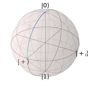
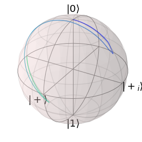
We can check the implementation of the coherent dynamics with a simple pulse:

x_pi_half_gate_pulse = np.zeros(shape=(n_time_steps, 2), dtype=float)
x_pi_half_gate_pulse[:, 0] = .25 * np.pi / (n_time_steps * delta_t)
x_pi_half_gate_pulse[:, 1] = .5 * np.pi
solver.set_optimization_parameters(x_pi_half_gate_pulse)
solver.plot_bloch_sphere()

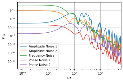
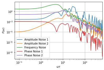
To get interesting filter functions, we generate a random pulse:

np.random.seed(4)
random_pulse = np.zeros(shape=(n_time_steps, 2), dtype=float)
random_pulse[:, 0] = np.random.rand(n_time_steps) * np.pi / (n_time_steps * delta_t)
random_pulse[:, 1] = 1 * np.random.rand(n_time_steps) * np.pi

solver.create_pulse_sequence(random_pulse)
pulse_sequence = solver.pulse_sequence
omega = ff.util.get_sample_frequencies(
    pulse_sequence, n_samples=200, spacing='log')
_ = ff.plotting.plot_filter_function(pulse_sequence, omega, yscale='log')

Now we define a noise spectral density. In our model, we assume that the amplitude is subjected to \(1/f\) type noise, the phase is subjected to white noise and the frequency is subjected to \(1/f^2\) noise.

We verify that everything is set up correctly by calculating the cost functions and compare the analytic to numeric derivatives calculated by finite differences.

def psd(f):
    spectral_power_density = np.zeros(shape=[5, f.shape[0]], dtype=float)
    # 1/f noise on the amplitudes
    spectral_power_density[0, :] = .01 / f
    spectral_power_density[1, :] = .01 / f
    # white noise on the phase
    spectral_power_density[2, :] = .1
    spectral_power_density[3, :] = .1
    # 1/f^2 noise on the frequency
    spectral_power_density[4, :] = .0001 / f ** 2
    return spectral_power_density

ff_infidelity = OperatorFilterFunctionInfidelity(
    solver=solver,
    noise_power_spec_density=psd,
    omega=omega
)

target_gate = DenseOperator.pauli_x().exp(-1j * .25 * np.pi)
coherent_infid = OperationInfidelity(
    solver=solver,
    target=target_gate
)

simulator = Simulator(
    solvers=[solver, ],
    cost_funcs=[coherent_infid, ff_infidelity]
)
print('Infidelities calculated with filter function:')
print(simulator.wrapped_cost_functions(random_pulse))
print('Absolute and relative deviation of analytic and numeric gradients.')
print(simulator.compare_numeric_to_analytic_gradient(random_pulse))

Infidelities calculated with filter function:
[0.81526447 0.00651779 0.02648523 0.00099263 0.00440001 0.04920558]
Absolute and relative deviation of analytic and numeric gradients.
(3.676565430814301e-08, 1.9975541347967917e-08)

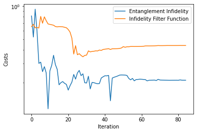
In a last step, we can start an optimization. We set the cost_func_weights to give the infidelitites calculated with the filter functions a higher weight of two orders of magnitude. This is sometimes necessary to avoid, that the optimizer simply optimizes the coherent dynamics and then gets stuck in a local optimum.

optimizer = ScalarMinimizingOptimizer(
    system_simulator=simulator,
    cost_func_weights=[1, 1e2, 1e2, 1e2, 1e2, 1e2]
)

result = optimizer.run_optimization(random_pulse)

data_container = DataContainer()
data_container.append_optim_result(result)
analyser = Analyser(data_container)
analyser.plot_costs()

<AxesSubplot:xlabel='Iteration', ylabel='Costs'>

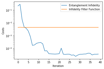
In a last step, we restart the optimization without weights to calibrate coherent errors. As initial pulse, we use the optimized pulse from the last optimization.

optimizer.cost_func_weights = None
result_2 = optimizer.run_optimization(result.final_parameters)
data_container.append_optim_result(result_2)
analyser.plot_costs(n=1)

solver.plot_bloch_sphere(result_2.final_parameters)
solver.create_pulse_sequence(result_2.final_parameters)
pulse_sequence = solver.pulse_sequence
_ = ff.plotting.plot_filter_function(pulse_sequence, omega, yscale='log')